3 Dynamics
Dynamics is the branch of mechanics that studies the motion of bodies under the action of forces. This chapter examines situations where forces produce acceleration, and it presents methods for analyzing the resulting motion, including the application of Newton’s laws, energy principles, and momentum conservation.
3.1 Inertia
Inertia is the property of a body that resists any change in its state of motion and is directly proportional to its mass. It can be understood as a form of “sluggishness” inherent to matter. For an object at rest, a net force is required to set it in motion; the greater the mass, the greater the force needed. Similarly, if an object is already moving, a net force is required to change its speed or direction, and the magnitude of this force is again proportional to the mass.
The term “inertia” is also used in structural mechanics to describe the resistance of a beam’s cross-section to bending, quantified by the second moment of area (see lecture notes on Second Moments).
3.2 Momentum
Momentum is the product of an object’s mass and its velocity and quantifies the amount of motion a moving body possesses. This concept is particularly important when considering a large vessel approaching a dock. Once the vessel is underway, its considerable momentum means that a substantial force, applied over sufficient time, is required to bring it to a stop or significantly alter its course. Without such intervention, the vessel will not stop quickly on its own and may collide with the dock.
3.3 Newton’s Laws of Motion
First Law (Law of Inertia):
An object remains at rest, or in uniform motion in a straight line, unless acted upon by a net external force.
\[ \Sigma F = 0 \implies v = \text{constant} \]Second Law (Law of Acceleration):
The acceleration of an object is directly proportional to the net force acting on it and inversely proportional to its mass.
\[ \vec{F} = m \vec{a} \]Third Law (Action-Reaction Law):
For every action, there is an equal and opposite reaction.
\[ \vec{F}_{\text{action}} = -\vec{F}_{\text{reaction}} \]
Example 3.1 Find the accelerating force required to increase the velocity of a body which has a mass of 20 kg from 30 m/s to 70 m/s in 4 s.
# Given

m = 20           # mass in kg
u = 30           # initial velocity in m/s
v = 70           # final velocity in m/s
t = 4            # time in seconds

# Calculate acceleration

a = (v - u) / t

# Calculate force

F = m * a

print(f"Acceleration: {a:.2f} m/s²")
print(f"Accelerating force: {F:.2f} N")
Example 3.2 A lift is supported by a steel wire rope, the total mass of the lift and contents is 750 kg. Find the tension in the wire rope, in newtons, when the lift is (i) moving at constant velocity, (ii) moving upwards and accelerating at 1.2 m/s2, (iii) moving upwards and retarding at 1.2 m/s2
# Given

m = 750          # mass in kg
g = 9.81         # gravitational acceleration in m/s^2

# Accelerations for each case

a_constant = 0
a_up_accel = 1.2
a_up_decel = -1.2

# Tension calculations

T_constant = m * (g + a_constant)
T_up_accel = m * (g + a_up_accel)
T_up_decel = m * (g + a_up_decel)

print(f"Tension at constant velocity: {T_constant:.4f} N")
print(f"Tension during upward acceleration: {T_up_accel:.4f} N")
print(f"Tension during upward deceleration: {T_up_decel:.4f} N")
3.4 Linear momentum
Linear momentum is a fundamental concept in physics that quantifies the motion of an object. It is defined as the product of the object’s mass and its velocity. Because momentum is a vector quantity, it possesses both magnitude and direction.
\[ Linear\ momentum = m \vec{v} \]
Where:
Linear momentum is in kg·m/s.
\(m\) is the mass of the object in kilograms.
\(\vec{v}\) is the velocity of the object in meters per second.
3.4.1 Conservation of Linear Momentum
The law of conservation of linear momentum states that, in a closed system with no external forces (or when the net external force is zero), the total linear momentum remains constant over time. This principle is particularly evident in collisions between two bodies. During a collision, the force exerted by the first body on the second is equal in magnitude and opposite in direction to the force exerted by the second on the first (Newton’s third law). These equal and opposite forces act for the same duration, producing changes in momentum that are equal in magnitude but opposite in direction. Consequently, the momentum gained by one body exactly equals the momentum lost by the other. Therefore, the total momentum of the system before the collision is equal to the total momentum after the collision.
In the absence of external forces, linear momentum is neither created nor destroyed; it is conserved. This is known as the law of conservation of linear momentum.
Example 3.3 A hand hammer with a head mass of 0.8 kg strikes a chisel at 9 m/s and comes to rest in 1/250 seconds. Calculate the average force exerted during the blow.
# Given

m = 0.8               # kg
u = 9                 # m/s (initial velocity)
v = 0                 # m/s (final velocity)
t = 1/250             # s (time to come to rest)

# Change in momentum

delta_p = m * (v - u)

# Average force

F_avg = delta_p / t

print(f"Average force during the blow: {F_avg:.4f} N")
Example 3.4 A jet of fresh water, 20 mm in diameter, emerges horizontally from a nozzle at a speed of 21 m/s and strikes a stationary vertical plate normally. Assuming no splashback (i.e., the water comes to rest upon impact with no velocity component normal to the plate after striking), calculate: (a) the mass flow rate of water leaving the nozzle (in kg/s), and (b) the force exerted by the jet on the plate. The density of fresh water is 1000 kg/m³.
import math

# Given

d = 0.02          # diameter in meters
v = 21            # jet speed in m/s
rho = 1000        # density of water in kg/m^3

# Mass flow rate

A = math.pi * (d**2) / 4        # cross-sectional area
v_dot = A * v                   # volumetric flow rate
m_dot = rho * v_dot             # mass flow rate

# Force on the plate

F = m_dot * v                   # momentum change

print(f"Mass flow rate (kg/s): {m_dot:.4f}")
print(f"Force on plate (N): {F:.4f}")
3.5 Angular Momentum
Angular momentum is the moment of linear momentum about a chosen point or axis. For a single particle, it is given by the cross product of its position vector (measured from that point) and its linear momentum.
More broadly, angular momentum measures the rotational motion of a system. For extended bodies, its evaluation depends on both the distance of mass elements from the axis (the first moment of position) and how the mass is distributed throughout the object—the moment of inertia, or second moment of mass.
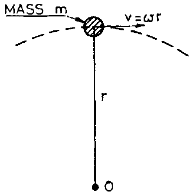
Given linear velocity \(\vec{v}\) and angular velocity \(\omega\):
\[ \vec{v} = r \omega \]
The linear momentum is determined by:
\[ \text{Linear momentum} = m \vec{v} \]
Substituting for \(\vec{v}\):
\[ \text{Linear momentum} = m r \omega \]
The moment of linear momentum can then be written as:
\[ \text{Moment of linear momentum} = m r \omega r \]
The moment of linear momentum is referred to as the angular momentum. Simplifying the above equation:
\[ \text{Angular momentum} = m r^2 \omega \]
Here, \(m r^2\) is the moment of inertia (second moment of mass) of the object about its axis of rotation, denoted as \(I\). Thus, the angular momentum can be expressed as:
\[ \text{Angular momentum} = I \omega \]
Where:
- \(I\) is the moment of inertia in \(kg·m²\).
- \(\omega\) is the angular velocity in \(rad/s\).
Additionally, the moment of inertia \(I\) is given by:
\[ I = m k^2 \]
Where:
- \(I\) is the moment of inertia in \(kg·m²\).
- \(m\) is the mass in \(kg\).
- \(k\) is the radius of gyration in \(m\).
In structural engineering, the moment of inertia (m⁴) is a measure of resistance to bending (deflection or stiffness).
In angular motion and physics, the moment of inertia (kg·m²) is a measure of resistance to angular acceleration (rotational inertia).
3.6 The Radius of Gyration
The radius of gyration is a geometric property of a rigid body or mass distribution that describes how the mass is distributed relative to an axis of rotation. It represents the effective distance from the axis at which the entire mass could be concentrated while producing the same moment of inertia as the actual distributed mass.
In simpler terms, a smaller radius of gyration means the mass is closer to the axis, which is good for reducing inertia in rotating machinery. This is desirable in applications like engine crankshafts or turbine rotors where rapid changes in speed are required. A larger radius of gyration means the mass is farther from the axis, like a hollow cylinder has a larger k than a solid cylinder of the same mass and outer radius. This is beneficial when energy storage is needed (e.g., flywheels).
Example 3.5 A flywheel of mass 500 kg and radius of gyration 1.2 m is running at 300 rev/min. By means of a clutch, this flywheel is suddenly connected to another flywheel, mass 2000 kg and radius of gyration 0.6 m, initially at rest. Calculate their common speed of rotation after engagement.
import math

# Given data

m1, k1 = 500, 1.2
m2, k2 = 2000, 0.6
rpm1 = 300

# Moments of inertia

I1 = m1 * k1**2
I2 = m2 * k2**2

# Convert rpm to rad/s

omega1 = (rpm1 / 60) * 2 * math.pi

# Conservation of angular momentum

omega_f = (I1 * omega1) / (I1 + I2)

# Convert rad/s to rpm

rpm_f = (omega_f / (2 * math.pi)) * 60

print(f"Final angular velocity (rad/s): {omega_f:.4f}")
print(f"Final angular velocity (rpm): {rpm_f:.4f}")
3.7 Turning Moment
We know the relation between linear acceleration \(a\) and angular acceleration \(\alpha\):
\[ a = r \alpha \]
And
\[ F = ma \]
Therefore,
\[ F = m \alpha r \]
If the force is not applied directly on the rim but at a greater or lesser leverage, say \(L\) from the centre, the effective force on the rim causing it to accelerate will be greater or lesser accordingly, in the ratio of \(L\) to \(r\). Thus:
\[ F \frac{L}{r} = m \alpha r \]
Multiplying both sides by \(r\),
\[ FL = m \alpha r^2 \]
Now, \(FL\) is the torque applied. Therefore, the accelerating torque is:
\[ \tau = m r^2 \alpha \]
Or,
\[ \tau = m k^2 \alpha \]
\(\tau\) is also given by:
\[ \tau = I \alpha \]
Where:
- \(\tau\) is the torque in \(Nm\).
- \(I\) is the moment of inertia in \(kg·m²\).
- \(\alpha\): Angular acceleration in \(rad/s^2\).
Example 3.6 The mass of a flywheel is 175 kg and its radius of gyration is 380 mm. Find the torque required to attain a speed of 500 rev/min from rest in 30 s.
import math

# Given
m = 175                 # mass in kg
k = 0.38                # radius of gyration in m
rpm_final = 500         # final speed
t = 30                  # time in seconds

# Moment of inertia
I = m * k**2

# Convert rpm → rad/s
omega_final = (rpm_final * 2 * math.pi) / 60

# Angular acceleration
alpha = omega_final / t

# Torque
tau = I * alpha

print(f"Moment of inertia I (kg·m^2): {I:.4f}")
print(f"Final angular velocity ω (rad/s): {omega_final:.4f}")
print(f"Angular acceleration α (rad/s^2): {alpha:.4f}")
print(f"Required torque τ (N·m): {tau:.4f}")
Example 3.7 The torque to overcome frictional and other resistances of a turbine is 317 N m and may be considered constant for all speeds. The mass of the rotating parts is 1.59 t and the radius of gyration is 0.686 m. If the gas is cut off when the turbine is running free of load at 1920 rev/min, find the time it will take to come to rest and the number of revolutions turned during that time.
import math

# Given

tau = 317.0           # N·m
m = 1.59 * 1000       # kg
k = 0.686             # m
rpm0 = 1920.0         # rev/min


I = m * k**2
omega0 = (rpm0 / 60.0) * 2.0 * math.pi   # rad/s
alpha = tau / I                          # rad/s^2
t = omega0 / alpha                       # s
theta = 0.5 * omega0 * t                 # rad
revs = theta / (2.0 * math.pi)


print(f"I (kg·m^2):           {I:.4f}")
print(f"omega0 (rad/s):       {omega0:.4f}")
print(f"alpha (rad/s^2):      {alpha:.6f}")
print(f"time to stop (s):     {t:.4f}")
print(f"time to stop (min):   {t/60:.4f}")
print(f"revolutions:          {revs:.4f}")
3.8 Power by Torque
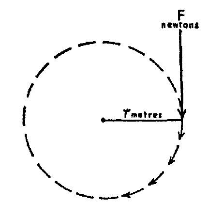
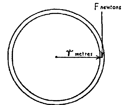
Consider a force \(F\) applied at a radius \(r\) on a rotating mechanism, as shown above.
The work done in one revolution is the product of the force and the circumference. Therefore:
\[ W = F \cdot 2 \pi r \]
If the mechanism is running at \(n\) revolutions per second:
\[ \text{Power} = F \cdot 2 \pi r n \]
Since torque \(\tau = F r\), we can rewrite the equation as:
\[ P = \tau \cdot 2 \pi n \]
Given that \(\omega = 2 \pi n\):
\[ P = \tau \cdot \omega \]
Where:
- \(P\) is the power in watts (W),
- \(\tau\) is the torque in newton-meters (Nm), and
- \(\omega\) is the angular velocity in radians per second (rad/s).
Example 3.8 The mean torque in a propeller shaft is 2.26 x 10⁵ Nm when running at 140 rpm. Find the power transmitted.
import math

# Given

T = 2.26e5      # Nm
rpm = 140

omega = rpm * 2 * math.pi / 60
P = T * omega

print(f"Angular speed (rad/s): {omega:.4f}")
print(f"Power (W): {P:.4f}")
print(f"Power (MW): {P/1e6:.4f}")
Example 3.9 One gear wheel with 100 teeth of 6 mm pitch running at 250 rev/min drives another which has 50 teeth. If the power transmitted is 0.5 kW, find the driving force on the teeth and the speed of the driven wheel.
import math

# Given

N1 = 100          # teeth on driving wheel
N2 = 50           # teeth on driven wheel
pitch = 0.006     # circular pitch (m)
n1 = 250          # driving rpm
P = 0.5e3         # power in watts

# Pitch diameter of driving wheel

D1 = (N1 * pitch) / math.pi
r1 = D1 / 2

# Angular speed of driving wheel

omega1 = n1 * 2 * math.pi / 60

# Torque on driving wheel

T = P / omega1

# Tangential driving force

F = T / r1

# Driven wheel speed

n2 = n1 * (N1 / N2)

print(f"Pitch diameter D1 (m): {D1:.4f}")
print(f"Torque T (N·m): {T:.4f}")
print(f"Tangential force F (N): {F:.4f}")
print(f"Driven wheel speed n2 (rpm): {n2:.4f}")
3.9 Kinetic Energy of Rotation
We know that \(K.E. = \frac{1}{2}mv^2\), where \(v\) is the linear velocity of the body. For a rotating body, the effective linear velocity is at the radius of gyration, as this is the radius at which the entire mass of the rotating body can be considered to act.
Let \(k\) = radius of gyration (in meters),
Let \(\omega\) = angular velocity (in radians per second).
The relationship between linear and angular velocity is:
\[ v = \omega k \]
Substituting \(v^2 = \omega^2 k^2\) into \(K.E. = \frac{1}{2}mv^2\) gives:
\[ \text{Rotational K.E.} = \frac{1}{2} m k^2 \omega^2 \]
Since \(I = m k^2\), where \(I\) is the moment of inertia:
\[ \text{Rotational K.E.} = \frac{1}{2} I \omega^2 \]
Example 3.10 The radius of gyration of the flywheel of a shearing machine is 0.46 m and its mass is 750 kg. Find the kinetic energy stored in it when running at 120 rev/min. If the speed falls to 100 rev/min during the cutting stroke, find the kinetic energy given out by the wheel.
import math

m = 750
k = 0.46
I = m * k**2

omega1 = 120 * 2 * math.pi / 60
omega2 = 100 * 2 * math.pi / 60

K1 = 0.5 * I * omega1**2
K2 = 0.5 * I * omega2**2
dK = K1 - K2

print(f"I (kg·m^2):           {I:.4f}")
print(f"KE at 120 rpm:        {K1/1e3:.4f} kJ")
print(f"KE at 100 rpm:        {K2/1e3:.4f} kJ")
print(f"Energy given out:     {dK/1e3:.4f} kJ")
Example 3.11 A ship’s anchor has a mass of 5 tonnes. Determine the work done in raising the anchor from a depth of 100 m. If the hauling gear is driven by a motor whose output is 80 kW and the efficiency of the haulage is 75%, determine how long the lifting operation takes.
# Given

m_anchor = 5 * 1000        # tonnes to kg
depth = 100                # m
g = 9.81                   # m/s^2

motor_power = 80_000       # W
efficiency = 0.75          # 75%

# Work done lifting the anchor

work_done = m_anchor * g * depth

# Effective power available for lifting

useful_power = motor_power * efficiency

# Time required

time_seconds = work_done / useful_power

print("Work done in lifting the anchor (MJ): {:.4f}".format(work_done/1e6))
print("Time required (s): {:.4f}".format(time_seconds))
4 Summary of Key Terms
4.0.1 Inertia
The tendency of an object to resist any change in its motion. An object with greater mass has greater inertia (it is “harder to start or stop”).
- In Naval Architecture, the moment of inertia (units: m⁴) is a measure of resistance to bending (related to stiffness/deflection of beams and hull girders).
- In angular motion and physics, the moment of inertia (units: kg·m²) is a measure of resistance to angular acceleration (rotational inertia).
4.0.2 Linear Momentum (p)
Momentum is the “quantity of motion” an object has. It is calculated as:
\[p = m v\]
where
- \(p\) = linear momentum (kg·m/s)
- \(m\) = mass (kg)
- \(v\) = velocity (m/s)
Momentum is a vector quantity (it has both magnitude and direction).
4.0.3 Newton’s Laws of Motion
4.0.3.1 First Law (Law of Inertia)
An object will stay at rest or keep moving in a straight line at constant speed unless an unbalanced (net) external force acts on it.
4.0.3.2 Second Law (Law of Acceleration)
The acceleration of an object is directly proportional to the net force acting on it and inversely proportional to its mass.
\[F_{\text{net}} = m a \quad \text{or} \quad a = \frac{F_{\text{net}}}{m}\]
4.0.3.3 Third Law (Action-Reaction)
Whenever two objects interact, they exert equal and opposite forces on each other.
“For every action force, there is an equal and opposite reaction force.”
4.0.4 Conservation of Linear Momentum
If no external forces act on a system (or if the external forces cancel out), the total momentum of the system stays constant.
In collisions or explosions:
Total momentum before = Total momentum after
Example: When two objects collide and stick together or bounce apart, the momentum lost by one is exactly gained by the other, so the total remains the same.
4.0.5 Angular Momentum
The rotational equivalent of linear momentum. It describes how much “rotational motion” a spinning or orbiting object has.
Angular momentum depends on mass, speed, and distance from the axis of rotation.
4.0.6 Radius of Gyration (k)
A geometric property of a rigid body that indicates how the mass is distributed relative to a specified axis of rotation. It is defined such that:
\[I = m k^2\]
where
- \(I\) = moment of inertia (kg·m²)
- \(m\) = total mass (kg)
- \(k\) = radius of gyration (m)
4.0.6.1 Practical Examples for Radius of Gyration
Smaller \(k\) → mass is concentrated closer to the axis → lower rotational inertia
→ easier/faster to speed up or slow down rotation
(e.g., engine crankshafts, turbine rotors, figure skater pulling arms in).Larger \(k\) → mass is distributed farther from the axis → higher rotational inertia
→ better for storing rotational energy
(e.g., flywheels; a hollow cylinder has a larger \(k\) than a solid cylinder of the same mass and outer radius).